Introduction to LSM Trees
Aren’t B-Trees good enough?
It is common knowledge that B+-Trees are the go-to data structure for SQL database indexes. They provide impressive log(n) read and write performance. However, one of their main drawbacks is that they require random I/O for disk reads across B-tree nodes, in order to update data in place.
Log-Structured Merge (LSM) Trees exploit sequential I/O to provide blazing fast write performance for KV databases, using insights from “Append Only” file systems. They are widely used in popular distributed dbs like Cassandra, ScyllaDB etc.
Let’s dive into how they work.
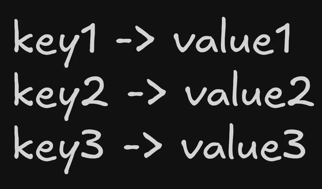
The simplest KV store possible
The world’s simplest KV store, just has all key value pairs stored in a file sequentially.
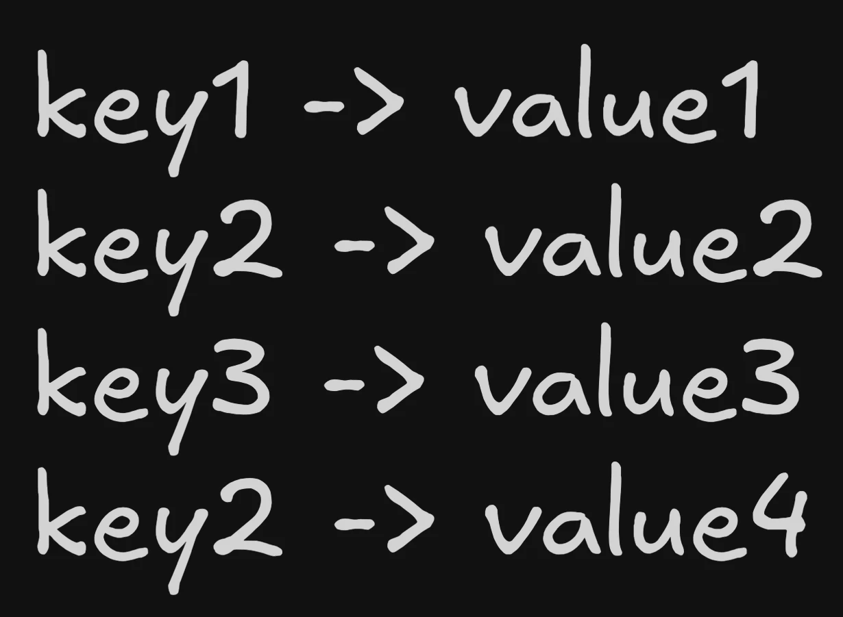
Updating gets a little tricky though, we have to scan through the file, find the key and update the value in place. That would require a bunch of reads before writing, making writes quite slow.
Taking inspiration from append only logs, we can just append the new key value pair to the bottom of the file. Then during reads, we scan from bottom to top and the first instance we find has the latest value! Below we change the value of key2 to value4 by appending.
This is the basic principle behind LSM Trees - Using append only sequential writes to make writes blazing fast!
Let’s look at how this is implemented for real now.
The Memtable
It starts off pretty simple - an in-memory data structure where we do in place reads and writes. For deletes - we use a special tombstone marker. For durability, all operations are first written to a WAL (Write Ahead Log) on disk. The only function of this is to recover the memtable if the DB crashes.
Memtable
In-Memory RB Tree/Skip List
SSTables
When the memtable reaches a certain threshold, we flush the data to disk, ensuring that the keys are sorted. This flush is done using sequential I/O, making it very fast. This on-disk structure is called an Sorted String Table (SSTable). After flushing we clear out the memtable and start fresh.
Each SSTable contains:
- Data blocks: The actual key-value pairs, sorted by key
- Index: A sparse index pointing to data block offsets
- Bloom filter: A probabilistic data structure to quickly check if a key might exist
SSTable
Flush to disk with sorted keys
How are reads handled?
As writes keep happening multiple SSTables accumulate on disk. To read a key, we search from newest to oldest:
- Check the memtable first (newest data)
- For each SSTable (newest to oldest):
- Check the bloom filter - if it says “no”, skip this SSTable
- If bloom filter says “maybe”, search the index to find the right block
- Scan the block to find the key
The latest value always wins - finding a tombstone means that the key was deleted.
SSTable Reads
How reads work in SSTables
Compaction
Reads sound quite expensive, we have to look at every SSTable! There is also a lot of redundant data across SSTables - i.e multiple versions of the same key. We only really need the latest version. To solve these issues, in a background job, we merge SSTables together using the familiar merge sort algorithm, and discard obsolete data (we keep tombstones though!). This reduces the number of SSTables we have to scan during reads.
Compaction
How SSTables are merged
This doesn’t look like a tree?
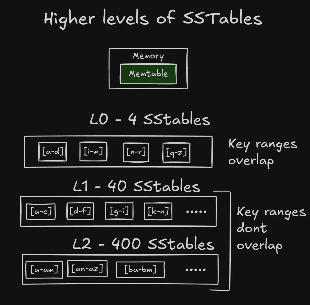
The above description is only describing a single level of SSTables called L0 - which represent recent writes/updates.
We limit the number of SSTables in L0 to a small number (usually 4) as we need to search all of them for reads.
When more than 4 SSTables accumulate in L0, we compact them into the next level - L1.
L1 and higher levels are where things get interesting -> while compacting we ensure that SSTables have disjoint key ranges. What happens when there are too many SSTables in L1? We compact them into L2, and so on.
Compactions across levels
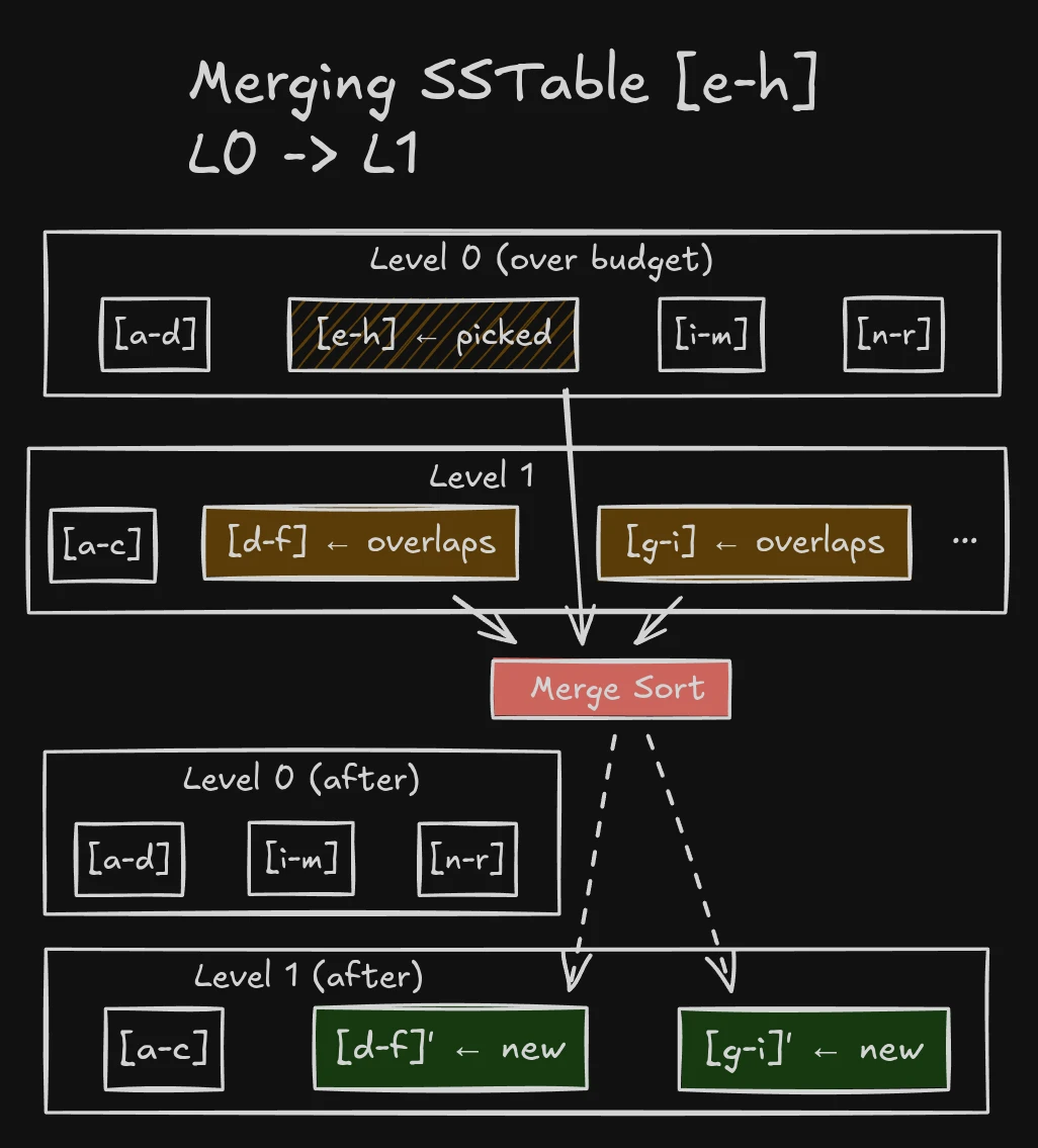
The compaction process checks the next level for SSTables with overlapping key ranges, and merges them together.
For L0 to L1 compactions, we usually have to merge all L1 SSTables with the L0 SSTable because L0 SSTables can have overlapping key ranges.
Since there are exponentially more SSTables in L2 than L1, each SSTable covers a smaller key range.
For L1 to L2 compactions (and higher levels), since all SSTables have disjoint key ranges, we only need to merge the SSTables in L2 whose range is a subset of the L1 SSTable being compacted.
Compactions are also much rarer at higher levels since they can store usually 10x more data than the previous level.
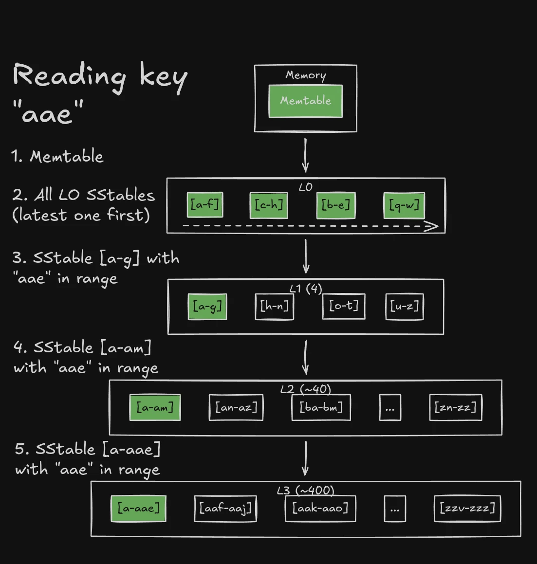
Reads across levels
When reading a key, the order of searching is:
- Memtable
- ALL L0 SSTables (newest to oldest)
- L1 SStable with the key in its range
- L2 SStable with the key in its range
- And so on…
This is why we keep tombstones during compactions! If we didn’t, we could read an older SSTable entry with a stale value! We end up reading quite a few SSTables in the worst case - this is called read amplification, where 1 read can turn into multiple disk reads as we search SSTables.
Write performance
If you noticed, almost all writes use sequential I/O - including memtable flushes and compactions. This is what allows DBs like Cassandra to not break a sweat under ridiculously high write load.
However, unlike BTrees which update in place - the same key may be present in multiple SSTables across levels. This is called write amplification, where 1 logical write can turn into multiple disk writes.
What’s left?
There are still a whole host of topics I hope to cover in future posts:
- Different compaction strategies (Size Tiered, Leveled, Universal)
- Range queries
- Why tombstones are hard to remove
- How reads/writes are served during compactions
Hope you enjoyed this introductory post, and stay tuned for more!